Run the cavity case and post-process its time directories

By the end of this tutorial you will have:

• truncated the cavity’s runtime by editing system/controlDict (the modify-and-write pattern from Read, modify, and write OpenFOAM dictionaries),

• driven OpenFOAM’s icoFoam PISO loop to completion from Python with one call to solver.run(),

• opened the resulting case with pyvista, iterated the written time directories, and sampled velocity on the cavity’s vertical mid-line, and

• plotted the family of |U|(y) profiles colour-coded by time.

The skill on display is the canonical CFD workflow: run the simulation, then post-process the on-disk results. Sampling lives after the time loop, not inside it.

Prerequisites

• Finished Modify initial conditions of the cavity case.

• The icoFoam solver class lives in examples/cavity/icoFoam.py; we import it directly.

Clone the case

from pybFoam import clone_example

case = clone_example("cavity")
print(f"case = {case}")

case = /tmp/pybfoam_2l1bzmul/cavity

Truncate the runtime

Default cavity endTime is 0.5 s — too long for a doc build. Shrink it and write at every step so we get one time directory per deltaT: t = 0.001, 0.002, …, 0.005.

from pybFoam import dictionary

control_dict_path = case / "system" / "controlDict"
cd = dictionary.read(str(control_dict_path))
cd.set("endTime", 0.005)
cd.set("deltaT", 0.001)
cd.set("writeInterval", 0.001)
cd.write(str(control_dict_path))

cd_check = dictionary.read(str(control_dict_path))
print("endTime       =", cd_check.get[float]("endTime"))
print("deltaT        =", cd_check.get[float]("deltaT"))
print("writeInterval =", cd_check.get[float]("writeInterval"))

endTime       = 0.005
deltaT        = 0.001
writeInterval = 0.001

Run the solver to completion

IcoFoam is shipped under examples/cavity/icoFoam.py. Tutorials are not on Python’s import path by default, so we add the cavity directory and import from it. pybFoam.examples_root() resolves the in-repo examples/ folder.

import sys

from pybFoam import examples_root

sys.path.insert(0, str(examples_root() / "cavity"))
from icoFoam import IcoFoam  # noqa: E402

solver = IcoFoam(case)
print(f"nCells = {solver.mesh.nCells()}   t0 = {solver.time.value()}")

solver.run()
print(f"finished at t = {solver.time.value()}")

nCells = 10000   t0 = 0.0
finished at t = 0.005

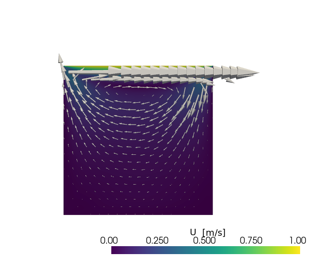
Snapshot the final state

Spatial context first — open the case with pybFoam.pyvista_read() and render a z-slice through the cavity slab at endTime with velocity glyphs. This shows where the vertical mid-line below cuts through the flow.

import pyvista as pv

from pybFoam import pyvista_read

L = 0.1  # cavity edge length
Z_MID = 0.5 * 0.01  # mid-z of the thin cavity slab

reader = pyvista_read(case)
all_times = sorted(t for t in reader.time_values if t > 0.0)

reader.set_active_time_value(all_times[-1])
internal_final = reader.read()["internalMesh"]
internal_final.set_active_vectors("U")
slice_mid = internal_final.slice(normal="z", origin=(0.5 * L, 0.5 * L, Z_MID))

plotter = pv.Plotter(window_size=(640, 540), off_screen=True)
plotter.add_mesh(
    slice_mid,
    scalars="U",
    cmap="viridis",
    show_edges=False,
    scalar_bar_args={"title": "|U|  [m/s]"},
)
plotter.add_mesh(
    slice_mid.glyph(orient="U", scale="U", factor=0.05, tolerance=0.04),
    color="white",
    line_width=1,
)
plotter.view_xy()
plotter.show()

Build an OpenFOAM sampler on the vertical mid-line

We want to sample with OpenFOAM’s own machinery (sampledSet + interpolation) rather than pyvista, since it gives the same interpolation OpenFOAM solvers use internally. The line is the canonical Ghia et al. benchmark cut: vertical at x = L/2 from floor to lid, 50 evenly-spaced points.

A meshSearch is built once per mesh; the UniformSetConfig + sampledSet.New factory produces the polyline.

import numpy as np

from pybFoam import Word
from pybFoam.sampling import (
    UniformSetConfig,
    interpolationVector,
    meshSearch,
    sampledSet,
    sampleSetVector,
)

N = 50

search = meshSearch(solver.mesh)
line_cfg = UniformSetConfig(
    axis="distance",
    start=[0.5 * L, 0.0, Z_MID],
    end=[0.5 * L, L, Z_MID],
    nPoints=N,
)
line = sampledSet.New(Word("midLine"), solver.mesh, search, line_cfg.to_foam_dict())

distance = np.asarray(line.distance())
print(f"sample points : {len(distance)}   y range : {distance[0]:.3f} … {distance[-1]:.3f}")

sample points : 50   y range : 0.000 … 0.100

Iterate the written time directories

pybFoam.selectTimes() enumerates every time directory under the case as a list of instant objects. For each we move the solver’s Time forward, load U from that time directory without registering it in the mesh (the still-live solver.U already occupies that name), and sample the line. The "cellPoint" interpolation scheme matches the default OpenFOAM sample utility.

from pybFoam import selectTimes, volVectorField

profiles: list[tuple[float, np.ndarray]] = []

for idx, inst in enumerate(selectTimes(solver.time, ["postProcess"])):
    t = float(str(inst))
    if t == 0.0:
        continue
    solver.time.setTime(inst, idx)
    U_t = volVectorField.read_field(solver.mesh, "U", register=False)
    interp = interpolationVector.New(Word("cellPoint"), U_t)
    sampled = np.asarray(sampleSetVector(line, interp))
    profiles.append((t, np.linalg.norm(sampled, axis=1)))

times = [t for t, _ in profiles]
print(f"sampled {len(profiles)} time steps × {N} points")

sampled 5 time steps × 50 points

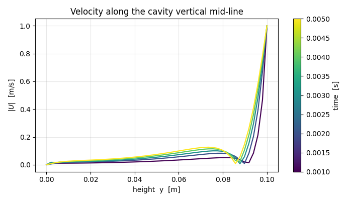
Plot the |U|(y) family

One curve per time step, coloured by physical time. The lid (y = L) drives the right-hand boundary; momentum diffuses downward as time progresses, raising the upper portion of every subsequent curve.

import matplotlib.pyplot as plt

fig, ax = plt.subplots(figsize=(7, 4))

norm = plt.Normalize(vmin=times[0], vmax=times[-1])
cmap = plt.get_cmap("viridis")

for t, u in profiles:
    ax.plot(distance, u, color=cmap(norm(t)), lw=1.6)

ax.set_xlabel("height  y  [m]")
ax.set_ylabel(r"$|U|$  [m/s]")
ax.set_title("Velocity along the cavity vertical mid-line")
ax.grid(alpha=0.3)

sm = plt.cm.ScalarMappable(cmap=cmap, norm=norm)
sm.set_array([])
fig.colorbar(sm, ax=ax, label="time  [s]")
fig.tight_layout()
plt.show()