Modify initial conditions of the cavity case

By the end of this tutorial you will have:

• read the cavity’s velocity field from 0/U,

• replaced its internal field with an analytic Taylor–Green–style vortex through a zero-copy NumPy view,

• written the modified field back to disk, and

• visualized the result with pyvista.

The skill on display is the round-trip: a NumPy edit lands inside the same buffer that OpenFOAM owns, and once pybFoam.write() serialises it, every downstream OpenFOAM tool — including pyvista’s OpenFOAMReader — sees the new state.

Prerequisites

• Finished Read, modify, and write OpenFOAM dictionaries and Build and operate on a scalarField.

• pybFoam installed with the [docs] extra (pyvista is required for the plot at the end).

Clone the case

from pybFoam import clone_example

case = clone_example("cavity")
print(f"case = {case}")

case = /tmp/pybfoam_8r1_ntkt/cavity

Build the mesh

The cavity ships only system/blockMeshDict; we generate the polyMesh explicitly so the meshing step is visible in the script. (T3 lets the solver class take care of this internally.)

from pybFoam import Time, argList, dictionary, fvMesh
from pybFoam.meshing import generate_blockmesh

time = Time(argList([str(case), "-case", str(case)]))
generate_blockmesh(time, dictionary.read(str(case / "system" / "blockMeshDict")))
mesh = fvMesh(time)

print(f"nCells = {mesh.nCells()}   nPoints = {mesh.nPoints()}")

nCells = 10000   nPoints = 20402

Read U

volVectorField.read_field opens <case>/0/U and returns a field whose internalField is exposed as a zero-copy buffer.

import numpy as np

from pybFoam import volVectorField

U = volVectorField.read_field(mesh, "U")
U_view = np.asarray(U["internalField"])

print(f"U.shape  = {U_view.shape}")
print(f"U[0]     = {U_view[0]}")
print(f"|U| max  = {np.linalg.norm(U_view, axis=1).max():.4f}  (uniform IC)")

U.shape  = (10000, 3)
U[0]     = [0. 0. 0.]
|U| max  = 0.0000  (uniform IC)

Build a Taylor–Green-style initial condition

fvMesh.C returns the cell-centre volVectorField. We pull it through NumPy and use the cell coordinates to evaluate an analytic divergence-free vortex on the (x, y) plane:

\[\begin{split}u_x &= \sin(\pi x/L)\,\cos(\pi y/L) \\ u_y &= -\cos(\pi x/L)\,\sin(\pi y/L)\end{split}\]

The cavity’s domain is \(L = 0.1\,\text{m}\).

L = 0.1  # cavity side length, from system/blockMeshDict (scale 0.1)

C = np.asarray(mesh.C()["internalField"])
x, y = C[:, 0], C[:, 1]

U_view[:, 0] = np.sin(np.pi * x / L) * np.cos(np.pi * y / L)
U_view[:, 1] = -np.cos(np.pi * x / L) * np.sin(np.pi * y / L)
U_view[:, 2] = 0.0

print(f"|U| max  = {np.linalg.norm(U_view, axis=1).max():.4f}  (after edit)")
print(f"|U| mean = {np.linalg.norm(U_view, axis=1).mean():.4f}")

|U| max  = 0.9998  (after edit)
|U| mean = 0.6775

Write U back to disk

The NumPy edit modified OpenFOAM’s owned memory in place; calling pybFoam.write() serialises the field — boundary conditions included — back into <case>/0/U.

from pybFoam import write

U.correctBoundaryConditions()
write(U)

written_U = (case / "0" / "U").read_text().splitlines()
nonuniform_lines = [i for i, line in enumerate(written_U) if "nonuniform" in line]
print(f"file lines        : {len(written_U)}")
print(f"'nonuniform' at line(s): {nonuniform_lines}")
# A successful round-trip turns the 'uniform (0 0 0)' entry into a
# 'nonuniform List<vector>' block. If you still see 'uniform' here,
# the write did not pick up the modified internalField.

file lines        : 10045
'nonuniform' at line(s): [20]

Visualize the modified IC

pybFoam.pyvista_read() wraps pyvista’s POpenFOAMReader so it reads the case directory we just wrote. We slice to the front face (z ≈ 0.005) to get a 2-D view and colour by |U|.

import pyvista as pv

from pybFoam import pyvista_read

reader = pyvista_read(case, time=0.0)
internal = reader.read()["internalMesh"]
internal.set_active_vectors("U")

slice_mid = internal.slice(normal="z", origin=(0.05, 0.05, 0.005))

plotter = pv.Plotter(window_size=(640, 540), off_screen=True)
plotter.add_mesh(
    slice_mid,
    scalars="U",
    cmap="viridis",
    show_edges=False,
    scalar_bar_args={"title": "|U|  [m/s]"},
)
plotter.add_mesh(
    slice_mid.glyph(orient="U", scale="U", factor=0.03, tolerance=0.04),
    color="white",
    line_width=1,
)
plotter.view_xy()
plotter.show()

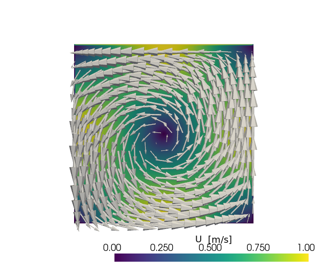
A successful edit shows a single rotating cell with stagnation at (L/2, L/2) and peak speed near the corners. A flat or noisy image would mean the NumPy edit never reached disk.