Sample a field along a line¶

Define a uniformly-spaced line with pybFoam.sampling.UniformSetConfig, create the set via sampledSet.New, and read scalar / vector values along it.

Tutorial T4 (Run the cavity case and post-process its time directories) shows how to do this inside a time loop. This page is the static (single-shot) version — useful for inspecting an existing result.

Prerequisite: a sourced OpenFOAM environment.

Set up case + mesh¶

from pybFoam import Time, argList, clone_example, dictionary, fvMesh
from pybFoam.meshing import generate_blockmesh

case = clone_example("case")
time = Time(argList([str(case), "-case", str(case)]))
generate_blockmesh(time, dictionary.read(str(case / "system" / "blockMeshDict")))
mesh = fvMesh(time)

Seed analytic `p_rgh`¶

The shipped IC for examples/case/ is uniform zero, which would leave the sampled line flat. We seed a sinusoidal pressure profile in place so the recipe has something to plot.

import numpy as np

from pybFoam import volScalarField, volVectorField, write

p_rgh_seed = volScalarField.read_field(mesh, "p_rgh")
U_seed = volVectorField.read_field(mesh, "U")

C = np.asarray(mesh.C()["internalField"])
L = 0.584  # case extent in x and y (scale 0.146 × 4)
np.asarray(p_rgh_seed["internalField"])[:] = (
    1000.0 * np.sin(np.pi * C[:, 0] / L) * np.sin(np.pi * C[:, 1] / L)
)
np.asarray(U_seed["internalField"])[:] = np.column_stack(
    [np.sin(np.pi * C[:, 1] / L), -np.sin(np.pi * C[:, 0] / L), np.zeros_like(C[:, 0])]
)
p_rgh_seed.correctBoundaryConditions()
U_seed.correctBoundaryConditions()
write(p_rgh_seed)
write(U_seed)

Define a uniform line¶

A meshSearch is required once per mesh and passed into every sampledSet.New call. The line endpoints below are in the scaled coordinate frame of examples/case/ (the dam-break geometry) and cross the central column at mid-height in z.

from pybFoam import Word
from pybFoam.sampling import UniformSetConfig, meshSearch, sampledSet

search = meshSearch(mesh)
cfg = UniformSetConfig(
    axis="distance",
    start=[0.1, 0.5, 0.005],
    end=[0.9, 0.5, 0.005],
    nPoints=50,
)
line = sampledSet.New(Word("xLine"), mesh, search, cfg.to_foam_dict())

print(f"points       : {line.nPoints()}")
print(f"axis         : {line.axis()}")

points       : 30
axis         : distance

Inspect the line geometry¶

points = np.asarray(line.points())
distance = np.asarray(line.distance())
cells = line.cells()

print(f"points.shape   : {points.shape}")
print(f"distance[0..3] : {distance[:3]}")
print(f"valid cells    : {sum(1 for c in cells if c >= 0)}/{len(cells)}")

points.shape   : (30, 3)
distance[0..3] : [0.         0.01632653 0.03265306]
valid cells    : 30/30

Interpolate a scalar field on the set¶

from pybFoam.sampling import OUT_OF_MESH, interpolationScalar, sampleSetScalar

p_rgh = p_rgh_seed  # already loaded and seeded above

interp = interpolationScalar.New(Word("cellPoint"), p_rgh)
sampled = sampleSetScalar(line, interp)

values = np.asarray(sampled)
# pybFoam.sampling.OUT_OF_MESH is the sentinel returned for sample
# points that did not land in any cell. Anything well below it is a
# real interpolated value.
valid_mask = values < OUT_OF_MESH / 10
valid_values = values[valid_mask]
print(f"p_rgh along xLine — min={valid_values.min():.3e}  max={valid_values.max():.3e}")

p_rgh along xLine — min=2.478e+01  max=4.364e+02

Reuse the same set for a vector field¶

A sampledSet is independent of the field — build it once, then drive multiple interpolators against it.

from pybFoam.sampling import interpolationVector, sampleSetVector

U = U_seed  # already loaded and seeded above

interp_U = interpolationVector.New(Word("cellPoint"), U)
sampled_U = sampleSetVector(line, interp_U)
U_values = np.asarray(sampled_U)
U_mag = np.linalg.norm(U_values, axis=1)
print(f"U along xLine shape: {U_values.shape}")

U along xLine shape: (30, 3)

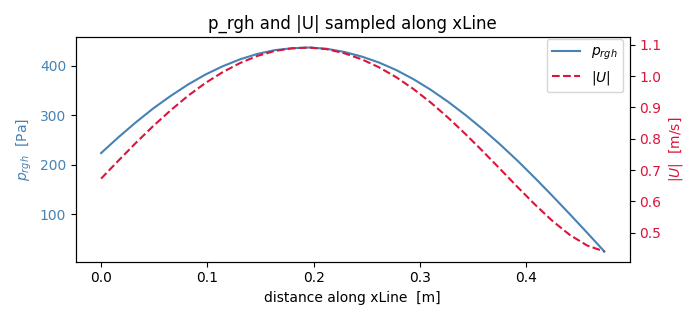
Plot the sampled line¶

Two y-axes: p_rgh on the left (matches the field magnitude), |U| on the right (so we can see both on the same x-axis even when the units differ). Off-mesh sentinel values are masked out.

import matplotlib.pyplot as plt

p_plot = np.where(valid_mask, values, np.nan)
u_plot = np.where(valid_mask, U_mag, np.nan)

fig, ax_p = plt.subplots(figsize=(7, 3.2))
(line_p,) = ax_p.plot(distance, p_plot, color="steelblue", label=r"$p_{rgh}$")
ax_p.set_xlabel("distance along xLine  [m]")
ax_p.set_ylabel(r"$p_{rgh}$  [Pa]", color="steelblue")
ax_p.tick_params(axis="y", labelcolor="steelblue")

ax_u = ax_p.twinx()
(line_u,) = ax_u.plot(distance, u_plot, color="crimson", label=r"$|U|$", linestyle="--")
ax_u.set_ylabel(r"$|U|$  [m/s]", color="crimson")
ax_u.tick_params(axis="y", labelcolor="crimson")

ax_p.set_title("p_rgh and |U| sampled along xLine")
fig.legend(handles=[line_p, line_u], loc="upper right", bbox_to_anchor=(0.9, 0.9))
fig.tight_layout()
plt.show()