Sample a field on an isosurface¶

An isosurface is the locus of cells where a field equals a chosen value. For VOF problems the natural example is the free surface alpha.water = 0.5. The factory pattern is the same one used for planes and patches — only the Pydantic config changes.

To get a non-trivial output without running a solver first, we seed analytic profiles for both the iso field (alpha.water) and the sampled field (p_rgh) through the zero-copy NumPy view, then let OpenFOAM’s sampledSurface.New extract the surface.

Prerequisite: finished Modify initial conditions of the cavity case and the Sample a field on a plane how-to.

Set up case + mesh¶

from pybFoam import Time, argList, clone_example, dictionary, fvMesh
from pybFoam.meshing import generate_blockmesh

case = clone_example("case")
time = Time(argList([str(case), "-case", str(case)]))
generate_blockmesh(time, dictionary.read(str(case / "system" / "blockMeshDict")))
mesh = fvMesh(time)

Seed analytic `alpha.water` and `p_rgh`¶

The shipped fields are uniform (the dam-break case relies on setFields to lay down water before launching). We seed them directly through the NumPy view so we can extract a meaningful iso surface here without needing the solver to run first.

import numpy as np

from pybFoam import volScalarField, write

alpha = volScalarField.read_field(mesh, "alpha.water")
p_rgh = volScalarField.read_field(mesh, "p_rgh")

C = np.asarray(mesh.C()["internalField"])
y = C[:, 1]

# Smooth alpha = 0.5 isosurface at y ≈ 0.2 (free-surface analogue).
alpha_view = np.asarray(alpha["internalField"])
alpha_view[:] = 0.5 * (1.0 - np.tanh((y - 0.2) * 50.0))

# Hydrostatic p_rgh below the interface, zero above.
rho_g = 1000.0 * 9.81  # kg/(m^2 s^2)
p_rgh_view = np.asarray(p_rgh["internalField"])
p_rgh_view[:] = np.maximum(rho_g * (0.2 - y), 0.0)

alpha.correctBoundaryConditions()
p_rgh.correctBoundaryConditions()
write(alpha)
write(p_rgh)

print(f"alpha range : {alpha_view.min():.3f} … {alpha_view.max():.3f}")
print(f"p_rgh range : {p_rgh_view.min():.3e} … {p_rgh_view.max():.3e} Pa")

alpha range : 0.000 … 1.000
p_rgh range : 0.000e+00 … 1.933e+03 Pa

Build the isosurface¶

SampledIsoSurfaceConfig validates the iso-field name and value at construction time. isoMethod="point" interpolates the iso field to mesh points before extracting the surface — gives the smoothest result.

from pybFoam import Word
from pybFoam.sampling import SampledIsoSurfaceConfig, sampledSurface

iso_cfg = SampledIsoSurfaceConfig(
    isoField="alpha.water",
    isoValue=0.5,
    isoMethod="point",
)
iso = sampledSurface.New(Word("waterSurface"), mesh, iso_cfg.to_foam_dict())
iso.update()

print(f"iso faces : {len(iso.magSf())}")
print(f"iso area  : {iso.area():.4f} m^2")

iso faces : 740
iso area  : 0.0085 m^2

Sample `p_rgh` on the isosurface¶

Same interpolationScalar + sampleOnFacesScalar pair used for planes and patches. The iso-surface is independent of the field being interpolated.

from pybFoam.sampling import interpolationScalar, sampleOnFacesScalar

interp = interpolationScalar.New(Word("cellPoint"), p_rgh)
sampled = sampleOnFacesScalar(iso, interp)

iso_centers = np.asarray(iso.Cf())
iso_values = np.asarray(sampled)
print(f"sampled shape : {iso_values.shape}")
print(
    f"p_rgh on iso  : min={iso_values.min():.3e}  "
    f"mean={iso_values.mean():.3e}  max={iso_values.max():.3e}"
)
# At y ≈ 0.2 the analytic hydrostatic p_rgh transitions through zero,
# so values close to zero confirm the surface really sits at the
# expected height.

sampled shape : (740,)
p_rgh on iso  : min=3.001e+01  mean=3.182e+01  max=3.692e+01

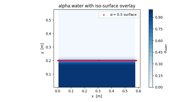
Plot the underlying alpha field with the iso-surface overlaid¶

Two layers: a tricontourf of alpha.water on the cell centres (background), and a scatter of iso.Cf() on top to show where the extracted surface sits. The case is 2-D (single z-layer), so a pure y-vs-x projection is enough.

import matplotlib.pyplot as plt

fig, ax = plt.subplots(figsize=(7, 4))
tcf = ax.tricontourf(C[:, 0], C[:, 1], alpha_view, levels=20, cmap="Blues")
fig.colorbar(tcf, ax=ax, label=r"$\alpha_\mathrm{water}$")

ax.scatter(
    iso_centers[:, 0],
    iso_centers[:, 1],
    c="crimson",
    s=8,
    label=r"$\alpha = 0.5$ surface",
)
ax.set_xlabel("x  [m]")
ax.set_ylabel("y  [m]")
ax.set_aspect("equal")
ax.set_title("alpha.water with iso-surface overlay")
ax.legend(loc="upper right")
fig.tight_layout()
plt.show()