Compute finite-volume operators from Python

pybFoam.fvc and pybFoam.fvm mirror OpenFOAM’s C++ operator API. fvc evaluates explicit operators and returns a tmp_* field wrapper; fvm produces implicit matrix terms that can be summed into an equation and solved.

This how-to evaluates every fvc operator the solver API exposes against the shipped VOF case, assembles a momentum matrix with fvm, and plots |∇p_rgh| on the cell centres.

Prerequisite: finished Build and operate on a scalarField.

Set up case + mesh

pybFoam.clone_example() copies the named example into a tmp dir and restores 0.orig → 0. The mesh is generated from system/blockMeshDict.

from pybFoam import Time, argList, clone_example, dictionary, fvMesh
from pybFoam.meshing import generate_blockmesh

case = clone_example("case")
time = Time(argList([str(case), "-case", str(case)]))
generate_blockmesh(time, dictionary.read(str(case / "system" / "blockMeshDict")))
mesh = fvMesh(time)
print(f"mesh: {mesh.nCells()} cells")

mesh: 2268 cells

Read fields

import numpy as np

from pybFoam import createPhi, volScalarField, volVectorField, write

p_rgh = volScalarField.read_field(mesh, "p_rgh")
U = volVectorField.read_field(mesh, "U")

# The shipped IC is uniform zero, which would leave grad / div / lap
# all at numerical noise. Seed an analytic sinusoidal pressure and a
# matching divergence-free velocity so the operator outputs are
# meaningful (and the gradient plot has visible structure).
C = np.asarray(mesh.C()["internalField"])
L = 0.584  # case extent (scale 0.146 × 4)
np.asarray(p_rgh["internalField"])[:] = (
    1000.0 * np.sin(np.pi * C[:, 0] / L) * np.sin(np.pi * C[:, 1] / L)
)
np.asarray(U["internalField"])[:] = np.column_stack(
    [np.sin(np.pi * C[:, 1] / L), -np.sin(np.pi * C[:, 0] / L), np.zeros_like(C[:, 0])]
)
p_rgh.correctBoundaryConditions()
U.correctBoundaryConditions()
write(p_rgh)
write(U)

phi = createPhi(U)

Explicit operators (fvc)

Each fvc call returns a tmp_* reference so OpenFOAM can reuse the underlying buffer — calling it (()) materialises the concrete field. Pass tmp_* directly into another operator to chain.

from pybFoam import fvc

grad_p = fvc.grad(p_rgh)()
div_U = fvc.div(U)()
lap_p = fvc.laplacian(p_rgh)()

print(f"grad(p_rgh) shape  : {np.asarray(grad_p['internalField']).shape}")
print(
    f"div(U)      min/max: "
    f"{np.asarray(div_U['internalField']).min():.3e} / "
    f"{np.asarray(div_U['internalField']).max():.3e}"
)
print(f"lap(p_rgh)  sum    : {np.asarray(lap_p['internalField']).sum():.3e}")

grad(p_rgh) shape  : (2268, 3)
div(U)      min/max: -1.678e+02 / 7.874e+01
lap(p_rgh)  sum    : 9.790e+06

Flux + surface-normal gradient + reconstruct

flux = fvc.flux(U)()  # surfaceScalarField
div_phiU = fvc.div(flux, U)()
snGrad_p = fvc.snGrad(p_rgh)()
reconstructed = fvc.reconstruct(flux)()

flux_vals = np.asarray(flux["internalField"])
snGrad_vals = np.asarray(snGrad_p["internalField"])
recon_vals = np.asarray(reconstructed["internalField"])

print(f"flux         : surfaceScalarField, {flux_vals.shape[0]} internal faces")
print(f"snGrad_p     : {snGrad_vals.shape[0]} internal face values")
print(f"reconstructed: volVectorField, {recon_vals.shape}")

flux         : surfaceScalarField, 4432 internal faces
snGrad_p     : 4432 internal face values
reconstructed: volVectorField, (2268, 3)

Implicit/matrix operators (fvm)

fvm operators produce terms of an equation matrix rather than field values. Combine them with + / - and wrap into an fvScalarMatrix or fvVectorMatrix.

from pybFoam import (
    Word,
    dimensionedScalar,
    dimLength,
    dimTime,
    fvm,
    fvScalarMatrix,
    fvVectorMatrix,
)

pEqn = fvScalarMatrix(fvm.laplacian(p_rgh))

nu = dimensionedScalar(Word("nu"), dimLength * dimLength / dimTime, 1.0e-5)
UEqn = fvVectorMatrix(fvm.ddt(U) + fvm.div(phi, U) - fvm.laplacian(nu, U))

print(f"pEqn: {type(pEqn).__name__}")
print(f"UEqn: {type(UEqn).__name__}")

pEqn: fvScalarMatrix
UEqn: fvVectorMatrix

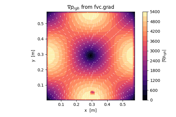
Visualize ∇p_rgh on the cell centres

mesh.C() gives the cell-centre volVectorField. Combined with np.asarray(grad_p['internalField']) we get a (n_cells, 3) array of the gradient and (n_cells, 3) cell coordinates. The case is 2-D (single layer in z), so a matplotlib tricontourf of the in-plane gradient magnitude is enough.

import matplotlib.pyplot as plt

C = np.asarray(mesh.C()["internalField"])
g = np.asarray(grad_p["internalField"])
mag_g = np.linalg.norm(g[:, :2], axis=1)

fig, ax = plt.subplots(figsize=(6, 4))
tcf = ax.tricontourf(C[:, 0], C[:, 1], mag_g, levels=20, cmap="magma")
fig.colorbar(tcf, ax=ax, label=r"$|\nabla p_{rgh}|$")

# Quiver on a coarse subsample so arrows are readable.
n_cells = C.shape[0]
step = max(1, n_cells // 400)
ax.quiver(
    C[::step, 0],
    C[::step, 1],
    g[::step, 0],
    g[::step, 1],
    color="white",
    scale=None,
    scale_units="xy",
    width=0.002,
)
ax.set_aspect("equal")
ax.set_xlabel("x  [m]")
ax.set_ylabel("y  [m]")
ax.set_title(r"$\nabla p_{rgh}$ from fvc.grad")
fig.tight_layout()
plt.show()

Mixing implicit and explicit terms

A typical PISO/SIMPLE loop builds the momentum matrix with fvm, adds an explicit pressure gradient from fvc, and hands the system to solve:

if piso.momentumPredictor():
    solve(UEqn + fvc.grad(p))

The shipped case uses p_rgh (full pressure) whose dimensions do not match UEqn, so we stop at showing the matrix shapes. For a worked solver see examples/cavity/icoFoam.py.

See also

• Run the cavity case and post-process its time directories — feed UEqn into the icoFoam PISO loop and sample the result.