Build and operate on a scalarField

By the end of this tutorial you will:

• construct a pybFoam.scalarField from a NumPy array,

• view it back as a NumPy array (zero-copy),

• apply OpenFOAM elementwise operators (sin, *, +, in-place +=) to it, and

• plot the result with matplotlib.

The point of this page is to show that scalarField is a real OpenFOAM primitive, not a NumPy wrapper. The same operators dispatch the same templated math that volScalarField uses inside a solver.

Prerequisites

• Finished Read, modify, and write OpenFOAM dictionaries.

Build a scalarField from NumPy

Constructing pybFoam.scalarField from a NumPy array copies the data into OpenFOAM’s memory once. From that point on, np.asarray(field) is a zero-copy view back to the same buffer — any in-place edit is visible to OpenFOAM.

import numpy as np

from pybFoam import scalarField

x = np.linspace(0.0, 1.0, 200)
field = scalarField(x)

print(f"len(field)        = {len(field)}")
print(f"np.asarray(field) = {np.asarray(field)[:5]} ...")

len(field)        = 200
np.asarray(field) = [0.         0.00502513 0.01005025 0.01507538 0.0201005 ] ...

Confirm zero-copy: edit through the view, see the update on the field side.

field_view = np.asarray(field)
field_view[0] = 99.0
print(f"field[0] after view edit = {field[0]}")
field_view[0] = x[0]  # restore

field[0] after view edit = 99.0

Elementwise operators are real OpenFOAM ops

Top-level functions like pybFoam.sin() take a scalarField and return a new one. +, -, *, / are bound directly, and there are in-place variants (+=, *=) too.

import pybFoam

y = pybFoam.sin(field * np.pi) * 2.0 + 1.0
y_np = np.asarray(y)

print(f"y range  : {y_np.min():.4f} … {y_np.max():.4f}")
print(f"y[50]    : {y_np[50]:.4f}   (analytic: {2 * np.sin(np.pi * x[50]) + 1:.4f})")

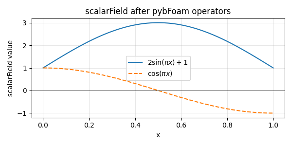
y range  : 1.0000 … 2.9999
y[50]    : 2.4198   (analytic: 2.4198)

The min should sit close to -1 (at \(x = 1.5/\pi\)) and the max close to 3 (at \(x = 0.5\)). The point-wise check at the middle of the range matches the analytic formula \(2\sin(\pi x) + 1\) to round-off — proof the operator chain evaluated and not just round-tripped.

In-place variants

Operators like += modify the field’s storage directly without allocating a new buffer.

z = scalarField(np.zeros_like(x))
z += pybFoam.cos(field * np.pi)
print(f"z[0]  = {np.asarray(z)[0]:.4f}   (cos 0 = 1)")
print(f"z[-1] = {np.asarray(z)[-1]:.4f}   (cos π = -1)")

z[0]  = 1.0000   (cos 0 = 1)
z[-1] = -1.0000   (cos π = -1)

Plot the result

A 1-D matplotlib line plot makes the shape of the operation obvious. A flat or zero curve here would mean an operator did not evaluate.

import matplotlib.pyplot as plt

fig, ax = plt.subplots(figsize=(6, 3))
ax.plot(x, y_np, label=r"$2\sin(\pi x) + 1$")
ax.plot(x, np.asarray(z), label=r"$\cos(\pi x)$", linestyle="--")
ax.axhline(0.0, color="k", lw=0.5)
ax.set_xlabel("x")
ax.set_ylabel("scalarField value")
ax.set_title("scalarField after pybFoam operators")
ax.legend()
ax.grid(alpha=0.3)
fig.tight_layout()
plt.show()