Run live with the solver, then plot

So far we drove execute / write by hand to keep tutorials self-contained. The whole point of pyOFTools, though, is that the running solver calls them for you. This tutorial closes the loop:

1. write a postProcess.py to the cloned case that combines the monitors from tutorials 02-04,

2. truncate the case’s endTime so the run completes in seconds,

3. run compressibleInterFoam — OpenFOAM picks up the pyPostProcessing function object from system/controlDict and calls the registered @Table outputs on every step,

4. load the resulting CSVs with pandas and plot the time-series.

The wiring in system/controlDict is already there in the damBreak case — see Your first in-situ post-processor for the snippet.

Clone the case

import os
import subprocess

import numpy as np  # noqa: F401  — imported early to dodge SIGFPE

import pyOFTools.patch_pybfoam  # noqa: F401
from pyOFTools import clone_example

CASE = clone_example("damBreak")
print(f"working case: {CASE}")

working case: /tmp/pyoftools_vu416hp1/damBreak

The post-processor file

OpenFOAM’s pyPostProcessing function object imports postProcess.py from the case directory, calls the module-level postProcess object with the mesh to get a runner, then calls execute / write / end on it. The damBreak case already ships such a file, and clone_example brought it across with the rest of the case:

examples/damBreak/postProcess.py

"""In-situ monitors for the damBreak case.

Loaded by OpenFOAM's ``pyPostProcessing`` function object — see the
``pyPostProcessing`` block in ``system/controlDict``. The ``pyClassName``
there is ``postProcess``, so OpenFOAM looks up the module-level
``postProcess`` object below, calls it with the mesh to get a runner, and
drives ``execute`` / ``write`` / ``end`` on that runner on its own schedule.

Each ``@Table`` decorator below registers one CSV output. Add a new one and
the next run will produce a new file under ``postProcessing/`` — no other
plumbing needed.
"""

from pyOFTools.aggregators import Mean, Sum, VolIntegrate
from pyOFTools.binning import Directional
from pyOFTools.builders import area, field, iso_surface, plane, sample
from pyOFTools.postprocessor import PostProcessorBase

# ``base_path`` is concatenated with each filename verbatim, so it needs the
# trailing slash. Relative path → resolves under the solver's cwd, which is
# the case directory.
postProcess = PostProcessorBase(base_path="postProcessing/")


@postProcess.Table("water_volume.csv")
def water_volume(m):
    # Total volume of liquid in the tank — a conservation check.
    return field(m, "alpha.water") | VolIntegrate(name="water_volume")


@postProcess.Table("interface_area.csv")
def interface_area(m):
    # Area of the α = 0.5 iso-surface ≈ the gas–liquid interface. Grows when
    # the wave breaks up, drops when it coalesces.
    return iso_surface(m, "alpha.water", 0.5) | area() | Sum(name="interface_area")


@postProcess.Table("mass_profile_x.csv")
def mass_profile_x(m):
    # Mass binned along the tank's x-axis. ``rho`` only exists once the
    # thermophysical model has initialised, i.e. at the first solver step.
    edges = [0.0, 0.146, 0.292, 0.438, 0.584]
    return (
        field(m, "rho")
        | Directional(bins=edges, direction=(1.0, 0.0, 0.0), origin=(0.0, 0.0, 0.0))
        | VolIntegrate(name="mass")
    )


@postProcess.Table("mean_p_midplane.csv")
def mean_p_midplane(m):
    # Average pressure on a horizontal plane halfway up the initial water
    # column. ``sample`` interpolates the volume field onto the plane.
    return (
        plane(m, point=(0.0, 0.146, 0.0), normal=(0.0, 1.0, 0.0))
        | sample(m, "p")
        | Mean(name="mean_p_midplane")
    )

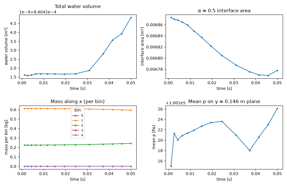
Four @Table outputs — water volume, interface area, mass profile along x, mean pressure on a horizontal mid-plane — combine the patterns from tutorials 02-04 into the single post-processor the live solver will call.

Trim endTime for the tutorial

The shipped controlDict runs to t = 2.0 — fine for a real study, too slow for a doc build. dictionary.read parses it, cd.set patches the entry, cd.write puts it back as a valid OpenFOAM dictionary (preserving format, comments, and adjacent entries).

from pybFoam import dictionary

control_dict_path = CASE / "system" / "controlDict"
cd = dictionary.read(str(control_dict_path))
cd.set("endTime", 0.05)
cd.write(str(control_dict_path))

Mesh, set fields, run the solver

Same sequence ./Allrun would do. The mesh is built in-process with generate_blockmesh; setFields and the solver run as subprocesses (the solver is a C++ binary, so no in-process equivalent).

from pybFoam import Time, argList, dictionary
from pybFoam.meshing import generate_blockmesh

env = {**os.environ}


def run(cmd):
    res = subprocess.run(cmd, cwd=CASE, env=env, capture_output=True, text=True, check=True)
    # OpenFOAM is chatty — show the tail so the gallery output stays useful.
    tail = "\n".join(res.stdout.splitlines()[-5:])
    print(f"$ {' '.join(cmd)}\n{tail}\n")


time = Time(argList([str(CASE), "-case", str(CASE)]))
generate_blockmesh(time, dictionary.read(str(CASE / "system" / "blockMeshDict")))
run(["pyoftools", "setFields", "system/setFields.py"])
run(["compressibleInterFoam"])

$ pyoftools setFields system/setFields.py
fileModificationChecking : Monitoring run-time modified files using timeStampMaster (fileModificationSkew 5, maxFileModificationPolls 20)
allowSystemOperations : Allowing user-supplied system call operations

// * * * * * * * * * * * * * * * * * * * * * * * * * * * * * * * * * * * * * //
I/O    : uncollated

$ compressibleInterFoam
        Viscous  : (-4.263073240876908e-06 -7.678422107909316e-05 6.094828253545187e-05)
    writing force and moment files.

End

Load the CSVs

Each @Table produced one CSV under postProcessing/. They have a time column plus the named value column (and group for binned outputs).

import pandas as pd

vol = pd.read_csv(CASE / "postProcessing" / "water_volume.csv")
area_df = pd.read_csv(CASE / "postProcessing" / "interface_area.csv")
mass = pd.read_csv(CASE / "postProcessing" / "mass_profile_x.csv")
plane_p = pd.read_csv(CASE / "postProcessing" / "mean_p_midplane.csv")

print(vol.head())
print(mass.head())

       time  water_volume
0  0.001190       0.00084
1  0.002626       0.00084
2  0.004318       0.00084
3  0.006304       0.00084
4  0.008732       0.00084
      time      mass  group
0  0.00119  0.000000      0
1  0.00119  0.612963      1
2  0.00119  0.224757      2
3  0.00119  0.001472      3
4  0.00119  0.001393      4

Plot the monitors

Four panels: water volume (should be conserved-ish), interface area (grows as the wave breaks up), per-bin mass along x (the wave front advances), and mean pressure on the mid-plane.

import matplotlib.pyplot as plt

fig, axes = plt.subplots(2, 2, figsize=(10, 6.5))

axes[0, 0].plot(vol["time"], vol["water_volume"], marker="o", markersize=3)
axes[0, 0].set(xlabel="time [s]", ylabel="water volume [m³]", title="Total water volume")

axes[0, 1].plot(area_df["time"], area_df["interface_area"], marker="o", markersize=3)
axes[0, 1].set(xlabel="time [s]", ylabel="interface area [m²]", title="α = 0.5 interface area")

# Long-format: one row per (time, bin). Pivot so each bin is its own line.
mass_wide = mass.pivot(index="time", columns="group", values="mass")
mass_wide.plot(ax=axes[1, 0], marker="o", markersize=3)
axes[1, 0].set(xlabel="time [s]", ylabel="mass per bin [kg]", title="Mass along x (per bin)")
axes[1, 0].legend(title="bin", fontsize=8)

axes[1, 1].plot(plane_p["time"], plane_p["mean_p_midplane"], marker="o", markersize=3)
axes[1, 1].set(xlabel="time [s]", ylabel="mean p [Pa]", title="Mean p on y = 0.146 m plane")

fig.tight_layout()
plt.show()

Visualise the interface at the final time

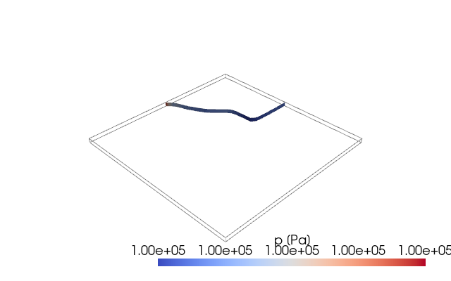
The CSVs only carry scalars; for the geometry of what just happened, drop back to pyvista. We pick the α = 0.5 iso-surface — the gas–liquid interface — at the end of the run and colour it by pressure.

import pyvista as pv
from pybFoam import pyvista_read

reader = pyvista_read(CASE)
reader.set_active_time_value(reader.time_values[-1])
internal = reader.read()["internalMesh"]
interface = internal.contour(isosurfaces=[0.5], scalars="alpha.water")

plotter = pv.Plotter(window_size=(640, 400), off_screen=True)
plotter.add_mesh(internal.outline(), color="gray")
plotter.add_mesh(
    interface,
    scalars="p",
    cmap="coolwarm",
    scalar_bar_args={"title": "p [Pa]"},
)
plotter.view_isometric()
plotter.show()

Where to go next

• How-to guides — point-in-time recipes for specific tasks (iso-surface area, residual extraction, custom aggregator).

• Wire pyOFTools into system/controlDict — full pyPostProcessing reference including writeControl variants and HDF5 output.

• Core data structures — what’s actually flowing through the pipeline (geometry, mask, groups, field) and how custom nodes fit in.