Your first in-situ post-processor

This is the shape pyOFTools is built for: a Python object that the running solver calls on every write step. You declare aggregates with PostProcessorBase + @Table, and the framework handles file lifecycle and CSV layout.

Here we’ll instrument the damBreak case with one monitor — the total volume of water — and watch a CSV row appear. We don’t run a solver here: we call the post-processor’s execute / write methods ourselves, exactly the way OpenFOAM’s pyPostProcessing function object would. Run live with the solver, then plot swaps the manual calls for a real live solver run.

Clone and prepare the case

Same setup as Set initial conditions with pyoftools setFields: clone, mesh, and run setFields so the field is non-uniform.

import subprocess

import numpy as np  # noqa: F401  — imported early to dodge SIGFPE

import pyOFTools.patch_pybfoam  # noqa: F401
from pyOFTools import clone_example

CASE = clone_example("damBreak")

Build the mesh and set initial fields

Same pre-processing as Set initial conditions with pyoftools setFields: generate_blockmesh writes the polyMesh, then the setFields CLI populates 0/alpha.water.

from pybFoam import Time, argList, dictionary, fvMesh, volScalarField
from pybFoam.meshing import generate_blockmesh

time = Time(argList([str(CASE), "-case", str(CASE)]))
generate_blockmesh(time, dictionary.read(str(CASE / "system" / "blockMeshDict")))
subprocess.run(
    ["pyoftools", "setFields", "system/setFields.py"],
    cwd=CASE,
    check=True,
    capture_output=True,
    text=True,
)

mesh = fvMesh(time)

# Pre-read fields so the post-processor finds them on the object registry.
volScalarField.read_field(mesh, "alpha.water")

<pybFoam.pybFoam_core.volScalarField object at 0x7f46decc9050>

Declare the post-processor

Three pieces:

1. PostProcessorBase(base_path=...) — a registry of named outputs.

2. @postProcess.Table(filename) — register a function that returns a WorkFlow. The framework calls it each write, hands it the mesh, and appends a CSV row.

3. Use name= on the aggregator to control the CSV column header.

Naming notes:

• base_path is concatenated with filename without a separator — include the trailing slash, and use an absolute path so the file lands inside the tmp case regardless of cwd.

• VolIntegrate(name="water_volume") gives a clean column name. Without it the column would be derived from the field name (alpha.water), which contains a dot pandas can stumble on.

from pyOFTools.aggregators import VolIntegrate
from pyOFTools.builders import field
from pyOFTools.postprocessor import PostProcessorBase

postProcess = PostProcessorBase(base_path=str(CASE) + "/postProcessing/")


@postProcess.Table("water_volume.csv")
def water_volume(m):
    return field(m, "alpha.water") | VolIntegrate(name="water_volume")

What that expression actually builds

field(m, "alpha.water") doesn’t compute anything yet — it returns a pyOFTools.workflow.WorkFlow: a lazy chain that carries a seed dataset (here, an InternalDataSet wrapping the field and the mesh geometry) plus an ordered list of nodes to apply. The pipe operator | appends a node and returns a new WorkFlow, so:

field(m, "alpha.water")  |  VolIntegrate(name="water_volume")
└────── seed ──────┘     └────── appended node ──────┘

Nothing runs until .compute() is called. The seed dataset flows through each node in order; each node returns a new (or in-place mutated) dataset for the next one. Selectors like Box write a mask onto the dataset, binners like Directional write groups, and reducers like VolIntegrate collapse the whole thing into an AggregatedDataSet. See Core data structures for the dataset taxonomy and the Protocol contract that makes all this composable.

Inside @postProcess.Table, you never call .compute() yourself — the framework does it each write step and turns the result into a CSV row. Outside the decorator (as the how-to recipes show), the same WorkFlow runs standalone via .compute().

Evaluate the post-processor at the current time step

Calling the PostProcessorBase with a mesh returns a runner that implements OpenFOAM’s function-object interface: execute() / write() / end(). We’re not running a solver in this tutorial — we call those methods ourselves to evaluate the pipeline on the initial fields and produce a single CSV row. That’s exactly what the live solver does each write step; Run live with the solver, then plot shows the controlDict wiring and a real solver run.

runner = postProcess(mesh)
runner.execute()
runner.write()
runner.end()

True

Inspect the output

One write call → one CSV row: a timestamp and the aggregated value.

import pandas as pd

csv_path = CASE / "postProcessing" / "water_volume.csv"
df = pd.read_csv(csv_path)
print(df)
water_volume_value = float(df["water_volume"].iloc[-1])

   time  water_volume
0   0.0       0.00084

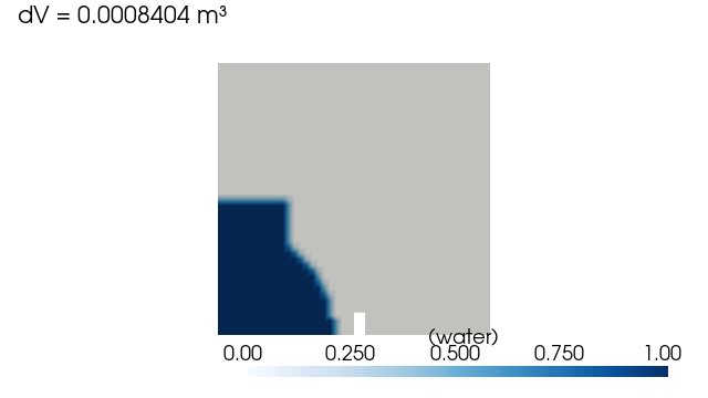
Visualise the field behind the number

The scalar in the CSV is the volume integral of the field we plot below — annotating the slice with the value ties the geometry to the number.

import pyvista as pv
from pybFoam import pyvista_read

reader = pyvista_read(CASE, time=0.0)
internal = reader.read()["internalMesh"]
slice_mid = internal.slice(normal="z", origin=(0.292, 0.292, 0.0075))

plotter = pv.Plotter(window_size=(640, 360), off_screen=True)
plotter.add_mesh(
    slice_mid,
    scalars="alpha.water",
    cmap="Blues",
    clim=(0.0, 1.0),
    scalar_bar_args={"title": "α (water)"},
)
plotter.add_text(
    f"∫ α dV = {water_volume_value:.4g} m³",
    position="upper_left",
    font_size=10,
)
plotter.view_xy()
plotter.show()

Next

• More monitors in the same post-processor — add a spatial profile and a region-restricted aggregate to the same class.

• Wire pyOFTools into system/controlDict — full controlDict reference for the pyPostProcessing function object.