Sample a field on a cutting plane

Interpolating a volume field onto a plane is the 2-D analogue of Sample a field along a line. You get back a SurfaceDataSet — face centres, face areas, and the sampled field. From there the usual reducers apply (Mean, Sum, SurfIntegrate).

Open the case

import os
import subprocess

import pyOFTools.patch_pybfoam  # noqa: F401
from pyOFTools import clone_example

CASE = clone_example("damBreak")
subprocess.run(
    ["./Allrun"],
    cwd=CASE,
    check=True,
    env={**os.environ},
    capture_output=True,
    text=True,
)

from pybFoam import Time, fvMesh, volScalarField

time = Time(str(CASE.parent), CASE.name)
mesh = fvMesh(time)
volScalarField.read_field(mesh, "p")

<pybFoam.pybFoam_core.volScalarField object at 0x7f46deccb790>

Sample p on a mid-plane

plane gives the geometry; sample(mesh, "p") interpolates p onto it.

from pyOFTools.aggregators import Max, Mean
from pyOFTools.builders import plane, sample

mid_plane_mean = (
    plane(mesh, point=(0.0, 0.292, 0.0), normal=(0, 1, 0)) | sample(mesh, "p") | Mean()
).compute()
print(f"mean p on y=0.292 plane = {mid_plane_mean.values[0].value:.4g} Pa")

mid_plane_max = (
    plane(mesh, point=(0.0, 0.292, 0.0), normal=(0, 1, 0)) | sample(mesh, "p") | Max()
).compute()
print(f"max  p on y=0.292 plane = {mid_plane_max.values[0].value:.4g} Pa")

mean p on y=0.292 plane = 1e+05 Pa
max  p on y=0.292 plane = 1e+05 Pa

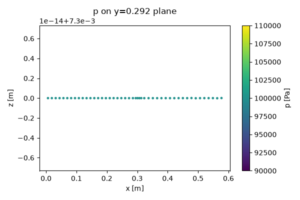
Scatter plot of sampled values

To inspect the field itself (not a reduction), compute() the plane workflow after sample but without a reducer — the returned object is the SurfaceDataSet with geometry and field populated.

from pyOFTools.workflow import WorkFlow

plane_wf = plane(mesh, point=(0.0, 0.292, 0.0), normal=(0, 1, 0)) | sample(mesh, "p")
assert isinstance(plane_wf, WorkFlow)
surface_ds = plane_wf.compute()

import matplotlib.pyplot as plt
import numpy as np

positions = np.asarray(surface_ds.geometry.positions)
p_values = np.asarray(surface_ds.field)

fig, ax = plt.subplots(figsize=(6, 4))
sc = ax.scatter(positions[:, 0], positions[:, 2], c=p_values, s=6)
ax.set_xlabel("x [m]")
ax.set_ylabel("z [m]")
ax.set_title("p on y=0.292 plane")
fig.colorbar(sc, ax=ax, label="p [Pa]")
fig.tight_layout()
plt.show()