More monitors in the same post-processor

One PostProcessorBase holds as many @Table outputs as you like. Each decorated function is an independent pipeline — they share the mesh and the write schedule, nothing else.

We’ll grow the post-processor from Your first in-situ post-processor by adding two more monitors:

• a water profile along the tank’s x-axis, using Directional binning;

• a region-restricted integral that drops a sphere from the domain, showing how the spatial selectors compose with & / | / ~.

We use alpha.water for the profile because it’s available before the solver runs. The natural choice — rho — only appears once the thermophysical model has initialised, which happens at the first solver step (see Run live with the solver, then plot for the live-solver version).

Clone, mesh, set fields

import subprocess

import numpy as np  # noqa: F401  — imported early to dodge SIGFPE

import pyOFTools.patch_pybfoam  # noqa: F401
from pyOFTools import clone_example

CASE = clone_example("damBreak")

from pybFoam import Time, argList, dictionary, fvMesh, volScalarField
from pybFoam.meshing import generate_blockmesh

time = Time(argList([str(CASE), "-case", str(CASE)]))
generate_blockmesh(time, dictionary.read(str(CASE / "system" / "blockMeshDict")))
subprocess.run(
    ["pyoftools", "setFields", "system/setFields.py"],
    cwd=CASE,
    check=True,
    capture_output=True,
    text=True,
)

mesh = fvMesh(time)
volScalarField.read_field(mesh, "alpha.water")

<pybFoam.pybFoam_core.volScalarField object at 0x7f46dff6ba50>

Declare the three outputs

Same pattern as before, three @Table registrations on one PostProcessorBase. Each will produce its own CSV under postProcessing/.

• water_volume — the monitor from tutorial 02, unchanged.

• water_profile_x — bin alpha.water along x, then integrate per bin. CSV has one row per bin per write with a group column for the bin id.

• water_outside_sphere — a Box & ~Sphere shell-region integral. Box and Sphere write masks; VolIntegrate honours them.

from pyOFTools.aggregators import VolIntegrate
from pyOFTools.binning import Directional
from pyOFTools.builders import field
from pyOFTools.postprocessor import PostProcessorBase
from pyOFTools.spatial_selectors import Box, Sphere

postProcess = PostProcessorBase(base_path=str(CASE) + "/postProcessing/")


@postProcess.Table("water_volume.csv")
def water_volume(m):
    return field(m, "alpha.water") | VolIntegrate(name="water_volume")


@postProcess.Table("water_profile_x.csv")
def water_profile_x(m):
    # 4 bins covering the tank along x (width = 0.584 m on damBreak).
    edges = [0.0, 0.146, 0.292, 0.438, 0.584]
    return (
        field(m, "alpha.water")
        | Directional(bins=edges, direction=(1.0, 0.0, 0.0), origin=(0.0, 0.0, 0.0))
        | VolIntegrate(name="water_per_bin")
    )


@postProcess.Table("water_outside_sphere.csv")
def water_outside_sphere(m):
    # Whole tank minus a sphere around the initial water column corner.
    region = Box(min=(0.0, 0.0, -1.0), max=(0.584, 0.584, 1.0)) & ~Sphere(
        center=(0.0, 0.0, 0.0), radius=0.2
    )
    return field(m, "alpha.water") | region | VolIntegrate(name="water_outside_sphere")

Evaluate at the current time step

Same pattern as tutorial 02 — we call execute / write ourselves on the initial fields instead of running a solver. The runner loops over every registered @Table and writes one row per CSV. Run live with the solver, then plot does the real in-situ run.

runner = postProcess(mesh)
runner.execute()
runner.write()
runner.end()

print("--- water_volume.csv ---")
print((CASE / "postProcessing" / "water_volume.csv").read_text())
print("--- water_profile_x.csv ---")
print((CASE / "postProcessing" / "water_profile_x.csv").read_text())
print("--- water_outside_sphere.csv ---")
print((CASE / "postProcessing" / "water_outside_sphere.csv").read_text())

--- water_volume.csv ---
time,water_volume
0.0,0.0008404216050726664

--- water_profile_x.csv ---
time,water_per_bin,group
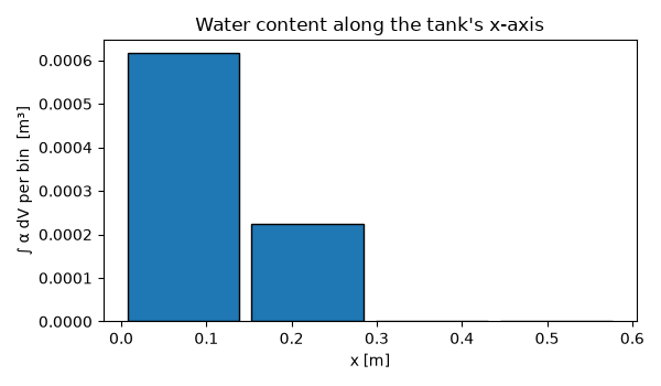
0.0,0.0,0
0.0,0.000615629573321276,1
0.0,0.000224792031751387,2
0.0,0.0,3
0.0,0.0,4

--- water_outside_sphere.csv ---
time,water_outside_sphere
0.0,0.00037858617683670325

Visualise the profile

A bar chart of per-bin water content shows where the water sits along x — the same information water_profile_x.csv carries, plotted.

import matplotlib.pyplot as plt
import pandas as pd

profile = pd.read_csv(CASE / "postProcessing" / "water_profile_x.csv")

# Drop the under/over-flow bins (group 0 and the last group): np.digitize
# uses those for "below the first edge" and "above the last edge".
interior = profile[(profile["group"] >= 1) & (profile["group"] <= 4)].copy()
bin_edges = [0.0, 0.146, 0.292, 0.438, 0.584]
bin_centres = [0.5 * (bin_edges[i - 1] + bin_edges[i]) for i in interior["group"]]
bin_width = bin_edges[1] - bin_edges[0]

fig, ax = plt.subplots(figsize=(6, 3.5))
ax.bar(bin_centres, interior["water_per_bin"], width=0.9 * bin_width, edgecolor="black")
ax.set_xlabel("x [m]")
ax.set_ylabel("∫ α dV per bin  [m³]")
ax.set_title("Water content along the tank's x-axis")
fig.tight_layout()
plt.show()

Visualise the sphere-excluded region

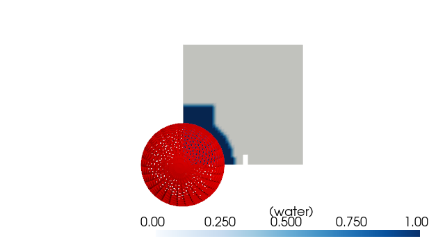
The Box & ~Sphere selector kept everything outside a sphere at the origin. Showing that sphere on a slice of the α field makes the geometric story explicit — the integral above came from cells outside it.

import pyvista as pv
from pybFoam import pyvista_read

reader = pyvista_read(CASE, time=0.0)
internal = reader.read()["internalMesh"]
slice_mid = internal.slice(normal="z", origin=(0.292, 0.292, 0.0075))

plotter = pv.Plotter(window_size=(640, 360), off_screen=True)
plotter.add_mesh(
    slice_mid,
    scalars="alpha.water",
    cmap="Blues",
    clim=(0.0, 1.0),
    scalar_bar_args={"title": "α (water)"},
)
# Outline of the excluded sphere on the same slice plane.
plotter.add_mesh(
    pv.Sphere(center=(0.0, 0.0, 0.0075), radius=0.2),
    color="red",
    style="wireframe",
    line_width=2,
    label="excluded sphere",
)
plotter.view_xy()
plotter.show()

What just happened

Three observations worth internalising:

• Per-bin rows: water_profile_x.csv has one row per bin per write, with the bin id in a group column. That’s how Directional reports profiles: tidy long-format, easy to load with pandas.

• Selectors compose with the pipeline: ... | region | VolIntegrate() reads naturally — the region is a node like any other, slotted in before the reducer.

• Selectors are dataset-agnostic: Box and Sphere only read positions and write mask, so the same expression works on volume fields, sampled surfaces, or line probes (see Core data structures).

Next: Surface monitors alongside volume ones — same class, with iso-surface area and a sampled pressure plane.