Surface monitors alongside volume ones

The post-processor doesn’t care whether the reducer feeds on volume cells, a sampled plane, or an iso-surface — it routes whatever the function returns through the same write step. This tutorial adds two surface-derived @Table outputs to the class we’ve been building:

• interface area — the area of the alpha.water = 0.5 iso-surface, a proxy for the gas–liquid interface,

• plane-averaged pressure — mean p on a horizontal cutting plane.

Both use the same builders documented in pyOFTools.builders.

Clone, mesh, set fields

import subprocess

import numpy as np  # noqa: F401  — imported early to dodge SIGFPE

import pyOFTools.patch_pybfoam  # noqa: F401
from pyOFTools import clone_example

CASE = clone_example("damBreak")

from pybFoam import Time, argList, dictionary, fvMesh, volScalarField
from pybFoam.meshing import generate_blockmesh

time = Time(argList([str(CASE), "-case", str(CASE)]))
generate_blockmesh(time, dictionary.read(str(CASE / "system" / "blockMeshDict")))
subprocess.run(
    ["pyoftools", "setFields", "system/setFields.py"],
    cwd=CASE,
    check=True,
    capture_output=True,
    text=True,
)

mesh = fvMesh(time)
volScalarField.read_field(mesh, "alpha.water")
volScalarField.read_field(mesh, "p")

<pybFoam.pybFoam_core.volScalarField object at 0x7f46e8efb310>

Two new builders

iso_surface(mesh, field, value) returns a workflow carrying just the iso-surface geometry — no field on it yet. Pipe into:

• area() to write face-area magnitudes onto the surface, then Sum to total them. That’s the “how much interface” number.

• sample(mesh, name) to interpolate a volume field onto the surface, then any reducer.

plane(mesh, point, normal) works the same way. We use it with sample + Mean for an area-weighted-free average pressure on a slice.

from pyOFTools.aggregators import Mean, Sum, VolIntegrate
from pyOFTools.builders import area, field, iso_surface, plane, sample
from pyOFTools.postprocessor import PostProcessorBase

postProcess = PostProcessorBase(base_path=str(CASE) + "/postProcessing/")


@postProcess.Table("water_volume.csv")
def water_volume(m):
    return field(m, "alpha.water") | VolIntegrate(name="water_volume")


@postProcess.Table("interface_area.csv")
def interface_area(m):
    return iso_surface(m, "alpha.water", 0.5) | area() | Sum(name="interface_area")


@postProcess.Table("mean_p_midplane.csv")
def mean_p_midplane(m):
    # Horizontal plane at y = 0.146 m, halfway up the initial water column.
    return (
        plane(m, point=(0.0, 0.146, 0.0), normal=(0.0, 1.0, 0.0))
        | sample(m, "p")
        | Mean(name="mean_p_midplane")
    )

Evaluate at the current time step

Same as before — we call execute / write on the initial fields instead of running a solver. Run live with the solver, then plot wires this class into controlDict and runs compressibleInterFoam so OpenFOAM does the calls for us.

runner = postProcess(mesh)
runner.execute()
runner.write()
runner.end()

import pandas as pd

results = {}
for name in ("water_volume.csv", "interface_area.csv", "mean_p_midplane.csv"):
    print(f"--- {name} ---")
    text = (CASE / "postProcessing" / name).read_text()
    print(text)
    df = pd.read_csv(CASE / "postProcessing" / name)
    results[name] = df.iloc[-1]

--- water_volume.csv ---
time,water_volume
0.0,0.0008404216050726664

--- interface_area.csv ---
time,interface_area
0.0,0.006872853348567688

--- mean_p_midplane.csv ---
time,mean_p_midplane
0.0,100000.0

Visualise the surfaces

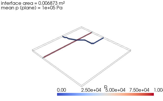
The two surface monitors are easier to read as 3-D geometry: the alpha = 0.5 iso-surface (the gas–liquid interface) and the horizontal cutting plane at y = 0.146 m (where we average pressure). pyvista extracts them from the same case and lets us draw them in one scene with the mesh outline for context.

import pyvista as pv
from pybFoam import pyvista_read

reader = pyvista_read(CASE, time=0.0)
internal = reader.read()["internalMesh"]
interface = internal.contour(isosurfaces=[0.5], scalars="alpha.water")
midplane = internal.slice(normal="y", origin=(0.292, 0.146, 0.0075))

plotter = pv.Plotter(window_size=(640, 400), off_screen=True)
plotter.add_mesh(internal.outline(), color="gray")
plotter.add_mesh(interface, color="royalblue", opacity=0.85, label="α = 0.5")
plotter.add_mesh(midplane, scalars="p", cmap="coolwarm", opacity=0.65)
plotter.add_text(
    f"interface area = {results['interface_area.csv']['interface_area']:.4g} m²\n"
    f"mean p (plane) = {results['mean_p_midplane.csv']['mean_p_midplane']:.4g} Pa",
    position="upper_left",
    font_size=10,
)
plotter.view_isometric()
plotter.show()

Takeaways

• iso_surface and plane give you a SurfaceDataSet; pipe into area() (face-area magnitudes) or sample(mesh, name) (interpolated volume field) before any reducer.

• Once the dataset is populated, the same reducers work everywhere — Mean / Sum / Min / Max on the surface, VolIntegrate on the volume. One vocabulary, many geometries.

• Box / Sphere selectors and Directional binners apply to surface datasets too (they only read positions).

Next: Run live with the solver, then plot — wire this class into the solver, run a real time window, and plot the resulting time-series.